Paso 1
a ) a) a )
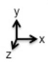
Para resolver esta pregunta, adoptaremos el sistema de coordenadas usual:
Recordando que una carga genérica q q q
E ⃗ = k ⋅ q r 2 r ^ \displaystyle \vec{E}=\frac{k \cdot q}{r^{2}} \hat{r} E = r 2 k ⋅ q r ^
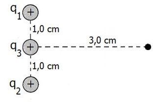
Solo resta analizar los tres casos, teniendo en cuenta que el campo eléctrico “sale” de las cargas positivas. Veamos la primera carga q 1 q_{1} q 1
Paso 2
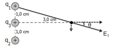
Para la carga q 1 q_{1} q 1 x x x y y y
E x → = ∣ E 1 ∣ ⋅ cos θ = ∣ E 1 ∣ ⋅ 3 3 2 + 1 2 i ^ \displaystyle \overrightarrow{E_{x}}=\left|E_{1}\right| \cdot \cos \theta=\left|E_{1}\right| \cdot \frac{3}{\sqrt{3^{2}+1^{2}}} \hat{i} E x = ∣ E 1 ∣ ⋅ cos θ = ∣ E 1 ∣ ⋅ 3 2 + 1 2 3 i ^
E y → = ∣ E 1 ∣ ⋅ sen θ = ∣ E 1 ∣ ⋅ 1 3 2 + 1 2 ( − j ^ ) \displaystyle \overrightarrow{E_{y}}=\left|E_{1}\right| \cdot \operatorname{sen} \theta=\left|E_{1}\right| \cdot \frac{1}{\sqrt{3^{2}+1^{2}}}(-\hat{j}) E y = ∣ E 1 ∣ ⋅ sen θ = ∣ E 1 ∣ ⋅ 3 2 + 1 2 1 ( − j ^ )
Para determinar el módulo de E 1 E_{1} E 1
∣ E ∣ = k ⋅ q r 2 \displaystyle |E|=\frac{k \cdot q}{r^{2}} ∣ E ∣ = r 2 k ⋅ q
∣ E 1 ∣ = 9 × 1 0 9 ⋅ 1 , 0 × 1 0 − 9 ( 3 2 + 1 2 × 1 0 − 2 ) 2 \displaystyle \left|E_{1}\right|=\frac{9 \times 10^{9} \cdot 1,0 \times 10^{-9}}{\left(\sqrt{3^{2}+1^{2}} \times 10^{-2}\right)^{2}} ∣ E 1 ∣ = ( 3 2 + 1 2 × 1 0 − 2 ) 2 9 × 1 0 9 ⋅ 1 , 0 × 1 0 − 9
∣ E 1 ∣ = 9 , 0 × 1 0 3 N / C \displaystyle \left|E_{1}\right|=9,0 \times 10^{3} N / C ∣ E 1 ∣ = 9 , 0 × 1 0 3 N / C
Ahora solo debemos sustituir y determinar las componentes
E x → = ∣ E 1 ∣ ⋅ 3 10 i ^ = 9 , 0 × 1 0 3 ⋅ 3 10 i ^ = 8 , 54 × 1 0 3 i ^ N / C \displaystyle \overrightarrow{E_{x}}=\left|E_{1}\right| \cdot \frac{3}{\sqrt{10}} \hat{i}=9,0 \times 10^{3} \cdot \frac{3}{\sqrt{10}} \hat{i}=8,54 \times 10^{3} \hat{i} N / C E x = ∣ E 1 ∣ ⋅ 10 3 i ^ = 9 , 0 × 1 0 3 ⋅ 10 3 i ^ = 8 , 54 × 1 0 3 i ^ N / C
E y → = ∣ E 1 ∣ ⋅ 1 10 ( − j ^ ) = 9 , 0 × 1 0 3 ⋅ 1 10 ( − j ^ ) = 2 , 85 × 1 0 3 ( − j ^ ) N / C \displaystyle \overrightarrow{E_{y}}=\left|E_{1}\right| \cdot \frac{1}{\sqrt{10}}(-\hat{j})=9,0 \times 10^{3} \cdot \frac{1}{\sqrt{10}}(-\hat{j})=2,85 \times 10^{3}(-\hat{j}) N / C E y = ∣ E 1 ∣ ⋅ 10 1 ( − j ^ ) = 9 , 0 × 1 0 3 ⋅ 10 1 ( − j ^ ) = 2 , 85 × 1 0 3 ( − j ^ ) N / C
La resultante E 1 → \overrightarrow{E_{1}} E 1
E 1 → = E x → + E y → \displaystyle \overrightarrow{E_{1}}=\overrightarrow{E_{x}}+\overrightarrow{E_{y}} E 1 = E x + E y
E 1 → = [ 8 , 54 × 1 0 3 i ^ + 2 , 85 × 1 0 3 ( − j ^ ) ] N / C \displaystyle \overrightarrow{E_{1}}=\left[8,54 \times 10^{3} \hat{i}+2,85 \times 10^{3}(-\hat{j})\right] N / C E 1 = [ 8 , 54 × 1 0 3 i ^ + 2 , 85 × 1 0 3 ( − j ^ ) ] N / C
Vayamos a la carga q 3 q_{3} q 3
Paso 3
Para q 3 q_{3} q 3 x x x
E 3 → = k ⋅ q r 2 i ^ = ( 9 , 0 × 1 0 9 ⋅ 1 , 0 × 1 0 − 9 ) ( 3 × 1 0 − 2 ) 2 i ^ = 1 , 0 × 1 0 4 i ^ N / C \displaystyle \overrightarrow{E_{3}}=\frac{k \cdot q}{r^{2}} \hat{i}=\frac{\left(9,0 \times 10^{9} \cdot 1,0 \times 10^{-9}\right)}{\left(3 \times 10^{-2}\right)^{2}} \hat{i}=1,0 \times 10^{4} \hat{i} N / C E 3 = r 2 k ⋅ q i ^ = ( 3 × 1 0 − 2 ) 2 ( 9 , 0 × 1 0 9 ⋅ 1 , 0 × 1 0 − 9 ) i ^ = 1 , 0 × 1 0 4 i ^ N / C
Llegó el turno de q 2 q_{2} q 2
Paso 4
Para q 2 q_{2} q 2 q 1 q_{1} q 1 y y y
E x → = ∣ E 2 ∣ ⋅ cos θ = ∣ E 2 ∣ ⋅ 3 3 2 + 1 2 i ^ \displaystyle \overrightarrow{E_{x}}=\left|E_{2}\right| \cdot \cos \theta=\left|E_{2}\right| \cdot \frac{3}{\sqrt{3^{2}+1^{2}}} \hat{i} E x = ∣ E 2 ∣ ⋅ cos θ = ∣ E 2 ∣ ⋅ 3 2 + 1 2 3 i ^
E y → = ∣ E 2 ∣ ⋅ sen θ = ∣ E 2 ∣ ⋅ 1 3 2 + 1 2 j ^ \displaystyle \overrightarrow{E_{y}}=\left|E_{2}\right| \cdot \operatorname{sen} \theta=\left|E_{2}\right| \cdot \frac{1}{\sqrt{3^{2}+1^{2}}} \hat{j} E y = ∣ E 2 ∣ ⋅ sen θ = ∣ E 2 ∣ ⋅ 3 2 + 1 2 1 j ^
Primero vamos a determinar ∣ E 2 ∣ \left|E_{2}\right| ∣ E 2 ∣
∣ E 2 ∣ = k ⋅ q r 2 = ( 9 , 0 × 1 0 9 ⋅ 1 , 0 × 1 0 − 9 ) ( 3 2 + 1 2 × 1 0 − 2 ) 2 = 9 , 0 × 1 0 3 N / C \displaystyle \left|E_{2}\right|=\frac{k \cdot q}{r^{2}}=\frac{\left(9,0 \times 10^{9} \cdot 1,0 \times 10^{-9}\right)}{\left(\sqrt{3^{2}+1^{2}} \times 10^{-2}\right)^{2}}=9,0 \times 10^{3} N / C ∣ E 2 ∣ = r 2 k ⋅ q = ( 3 2 + 1 2 × 1 0 − 2 ) 2 ( 9 , 0 × 1 0 9 ⋅ 1 , 0 × 1 0 − 9 ) = 9 , 0 × 1 0 3 N / C
Sustituyendo, tenemos:
E x → = 9 , 0 × 1 0 3 ⋅ 3 10 i ^ = 8 , 54 × 1 0 3 i ^ N / C \displaystyle \overrightarrow{E_{x}}=9,0 \times 10^{3} \cdot \frac{3}{\sqrt{10}} \hat{i}=8,54 \times 10^{3} \hat{i} N / C E x = 9 , 0 × 1 0 3 ⋅ 10 3 i ^ = 8 , 54 × 1 0 3 i ^ N / C
E y → = 9 , 0 × 1 0 3 ⋅ 1 10 j ^ = 2 , 85 × 1 0 3 j ^ N / C \displaystyle \overrightarrow{E_{y}}=9,0 \times 10^{3} \cdot \frac{1}{\sqrt{10}} \hat{j}=2,85 \times 10^{3} \hat{j} N / C E y = 9 , 0 × 1 0 3 ⋅ 10 1 j ^ = 2 , 85 × 1 0 3 j ^ N / C
La resultante E 2 → \overrightarrow{E_{2}} E 2
E 2 → = [ 8 , 54 × 1 0 3 i ^ + 2 , 85 × 1 0 3 j ^ ] N / C \displaystyle \overrightarrow{E_{2}}=\left[8,54 \times 10^{3} \hat{i}+2,85 \times 10^{3} \hat{j}\right] N / C E 2 = [ 8 , 54 × 1 0 3 i ^ + 2 , 85 × 1 0 3 j ^ ] N / C
Paso 5
b ) b) b )
Para hallar la resultante, debemos sumar los vectores que encontramos en los pasos anteriores.
E ⃗ r e s = E 1 → + E 2 → + E 3 → \displaystyle \vec{E}_{r e s}=\overrightarrow{E_{1}}+\overrightarrow{E_{2}}+\overrightarrow{E_{3}} E res = E 1 + E 2 + E 3
Sustituyendo, tenemos:
E ⃗ r e s = [ 8 , 54 × 1 0 3 i ^ + 2 , 85 × 1 0 3 ( − j ^ ) ] + 1 , 0 × 1 0 4 i ^ + [ 8 , 54 × 1 0 3 i ^ + 2 , 85 × 1 0 3 j ^ ] \displaystyle \vec{E}_{r e s}=\left[8,54 \times 10^{3} \hat{i}+2,85 \times 10^{3}(-\hat{j})\right]+1,0 \times 10^{4} \hat{i}+\left[8,54 \times 10^{3} \hat{i}+2,85 \times 10^{3} \hat{j}\right] E res = [ 8 , 54 × 1 0 3 i ^ + 2 , 85 × 1 0 3 ( − j ^ ) ] + 1 , 0 × 1 0 4 i ^ + [ 8 , 54 × 1 0 3 i ^ + 2 , 85 × 1 0 3 j ^ ]
E ⃗ r e s = 2 , 71 × 1 0 4 i ^ N / C \displaystyle \vec{E}_{r e s}=2,71 \times 10^{4} \hat{i} N / C E res = 2 , 71 × 1 0 4 i ^ N / C

 Continuar con Google